16  Bố trí thí nghiệm tối ưu hóa bằng R

16.0.1 Cơ sở lý thuyết về bố trí thí nghiệm tối ưu hóa

Phương pháp bề mặt đáp ứng (Response surface)

https://xdulieu.com/thiet-ke-thi-nghiem/tn5-be-mat-dap-ung/index.html

Hướng dẫn cách sử dụng package rsm để xử lý thí nghiệm tối ưu hóa

https://r-inthelab.net/2022/06/15/response-surface-designs-and-their-analysis-with-r/

16.0.2 Tình huống thường gặp

Bạn làm việc trong lĩnh vực công nghệ vi sinh, muốn tìm ra công thức nuôi cấy tế bào vi khuẩn tối ưu bằng phương pháp bề mặt đáp ứng (bố trí theo kiểu Box-Behnken design) với các yếu tố lần lượt là nhiệt độ, glucose, peptone, thời gian. Bình thường nếu làm trên Statgraphics thì cũng được, tuy nhiên giờ bạn muốn làm trên R thì như thế nào, có dễ thực hiện hay không.

Bạn tham khảo cách làm như sau nhé.

16.0.3 Cách thực hiện

Bước 1: Thiết kế thí nghiệm gồm 4 yếu tố, 3 mức để làm cơ sở cho bố trí thực nghiệm

library(rsm)

# Box-Behnken Design

bo_tri_thi_nghiem <- bbd(
    k  = 4,            # 4 yếu tố
    n0 = 3,            # 3 điểm trung tâm
    block = FALSE,     # No blocks 
    randomize = FALSE, # Not randomized
    coding = list(
        x1 ~ (nhiet_do - 40) / 5,
        x2 ~ (glucose - 100)/ 30,
        x3 ~ (peptone - 30) / 15,
        x4 ~ (thoi_gian - 24) / 12
    )
)

print(bo_tri_thi_nghiem)
   run.order std.order nhiet_do glucose peptone thoi_gian
1          1         1       35      70      30        24
2          2         2       45      70      30        24
3          3         3       35     130      30        24
4          4         4       45     130      30        24
5          5         5       40     100      15        12
6          6         6       40     100      45        12
7          7         7       40     100      15        36
8          8         8       40     100      45        36
9          9         9       35     100      30        12
10        10        10       45     100      30        12
11        11        11       35     100      30        36
12        12        12       45     100      30        36
13        13        13       40      70      15        24
14        14        14       40     130      15        24
15        15        15       40      70      45        24
16        16        16       40     130      45        24
17        17        17       35     100      15        24
18        18        18       45     100      15        24
19        19        19       35     100      45        24
20        20        20       45     100      45        24
21        21        21       40      70      30        12
22        22        22       40     130      30        12
23        23        23       40      70      30        36
24        24        24       40     130      30        36
25        25        25       40     100      30        24
26        26        26       40     100      30        24
27        27        27       40     100      30        24

Data are stored in coded form using these coding formulas ...
x1 ~ (nhiet_do - 40)/5
x2 ~ (glucose - 100)/30
x3 ~ (peptone - 30)/15
x4 ~ (thoi_gian - 24)/12

Bước 2: Thí nghiệm thực tế và đưa dữ liệu vào R

## Ở đây mình chạy số liệu mô phỏng về mật độ tế bào (log CFU/mL)

set.seed(14)
log_te_bao <- sample(seq(from = 3, to = 10, length.out= 1000), size = 27, replace = TRUE)

bo_tri_thi_nghiem$log_te_bao <- log_te_bao

print(bo_tri_thi_nghiem)
   run.order std.order nhiet_do glucose peptone thoi_gian log_te_bao
1          1         1       35      70      30        24   4.849850
2          2         2       45      70      30        24   8.885886
3          3         3       35     130      30        24   4.863864
4          4         4       45     130      30        24   5.599600
5          5         5       40     100      15        12   9.572573
6          6         6       40     100      45        12   8.262262
7          7         7       40     100      15        36   8.024024
8          8         8       40     100      45        36   6.006006
9          9         9       35     100      30        12   3.553554
10        10        10       45     100      30        12   6.048048
11        11        11       35     100      30        36   3.175175
12        12        12       45     100      30        36   6.461461
13        13        13       40      70      15        24   5.466466
14        14        14       40     130      15        24   6.419419
15        15        15       40      70      45        24   9.292292
16        16        16       40     130      45        24   5.431431
17        17        17       35     100      15        24   7.288288
18        18        18       45     100      15        24   3.686687
19        19        19       35     100      45        24   6.587588
20        20        20       45     100      45        24   3.735736
21        21        21       40      70      30        12   6.293293
22        22        22       40     130      30        12   9.138138
23        23        23       40      70      30        36   6.811812
24        24        24       40     130      30        36   4.268268
25        25        25       40     100      30        24   7.393393
26        26        26       40     100      30        24   7.512513
27        27        27       40     100      30        24   6.538539

Data are stored in coded form using these coding formulas ...
x1 ~ (nhiet_do - 40)/5
x2 ~ (glucose - 100)/30
x3 ~ (peptone - 30)/15
x4 ~ (thoi_gian - 24)/12

Bước 3: Tính toán model tối ưu hóa

ket_qua_model <- rsm(log_te_bao ~ SO(x1, x2, x3, x4), 
                   data = bo_tri_thi_nghiem)

summary(ket_qua_model)

Call:
rsm(formula = log_te_bao ~ SO(x1, x2, x3, x4), data = bo_tri_thi_nghiem)

             Estimate Std. Error t value  Pr(>|t|)    
(Intercept)  7.148148   1.061205  6.7359 2.086e-05 ***
x1           0.341592   0.530603  0.6438   0.53183    
x2          -0.489907   0.530603 -0.9233   0.37404    
x3          -0.095179   0.530603 -0.1794   0.86063    
x4          -0.676760   0.530603 -1.2755   0.22629    
x1:x2       -0.825075   0.919031 -0.8978   0.38697    
x1:x3        0.187437   0.919031  0.2040   0.84181    
x1:x4        0.197948   0.919031  0.2154   0.83308    
x2:x3       -1.203453   0.919031 -1.3095   0.21489    
x2:x4       -1.347097   0.919031 -1.4658   0.16842    
x3:x4       -0.176927   0.919031 -0.1925   0.85056    
x1^2        -1.720512   0.795904 -2.1617   0.05155 .  
x2^2        -0.147439   0.795904 -0.1852   0.85613    
x3^2         0.159117   0.795904  0.1999   0.84489    
x4^2        -0.110652   0.795904 -0.1390   0.89173    
---
Signif. codes:  0 '***' 0.001 '**' 0.01 '*' 0.05 '.' 0.1 ' ' 1

Multiple R-squared:  0.5306,    Adjusted R-squared:  -0.01707 
F-statistic: 0.9688 on 14 and 12 DF,  p-value: 0.528

Analysis of Variance Table

Response: log_te_bao
                    Df Sum Sq Mean Sq F value  Pr(>F)
FO(x1, x2, x3, x4)   4  9.885  2.4713  0.7315 0.58767
TWI(x1, x2, x3, x4)  6 16.197  2.6996  0.7990 0.58878
PQ(x1, x2, x3, x4)   4 19.742  4.9354  1.4608 0.27431
Residuals           12 40.542  3.3785                
Lack of fit         10 39.977  3.9977 14.1630 0.06771
Pure error           2  0.565  0.2823                

Stationary point of response surface:
        x1         x2         x3         x4 
 0.1775194 -0.4311620 -1.0998650  0.6045616 

Stationary point in original units:
 nhiet_do   glucose   peptone thoi_gian 
 40.88760  87.06514  13.50203  31.25474 

Eigenanalysis:
eigen() decomposition
$values
[1]  0.8592213  0.1237387 -0.9747800 -1.8276662

$vectors
         [,1]        [,2]       [,3]       [,4]
x1  0.1472489  0.03064641  0.2349074 0.96031092
x2 -0.6884443 -0.13747489 -0.6585456 0.27104034
x3  0.5555084 -0.71986015 -0.4143418 0.03914888
x4  0.4424620  0.67967846 -0.5826295 0.05298518

Bước 4: Vẽ đồ thị

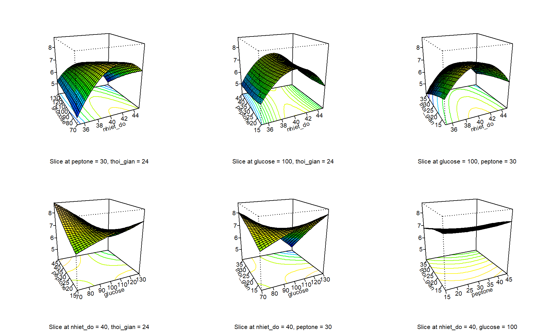
Thể hiện toàn bộ tương quan giữa các yếu tố với output mật độ tế bào

par(mfrow = c(2, 3))         # 2 x 3 pictures on one plot
persp(
    ket_qua_model,           # Our model
    ~ x1 + x2 + x3 + x4,     # A formula to obtain the 6 possible graphs
    col = topo.colors(100),  # Color palette
    contours = "colors",     # Include contours with the same color palette
    # xlabs = c("Nhiệt độ (°C)", 
    #           "Glucse (g/L)", 
    #           "Peptone (g/L)", 
    #           "Thời gian (giờ)" ), 
    # zlab = "Mật độ tế bào (log CFU/mL)",
    expand = 1,
    cex = 0.8
)

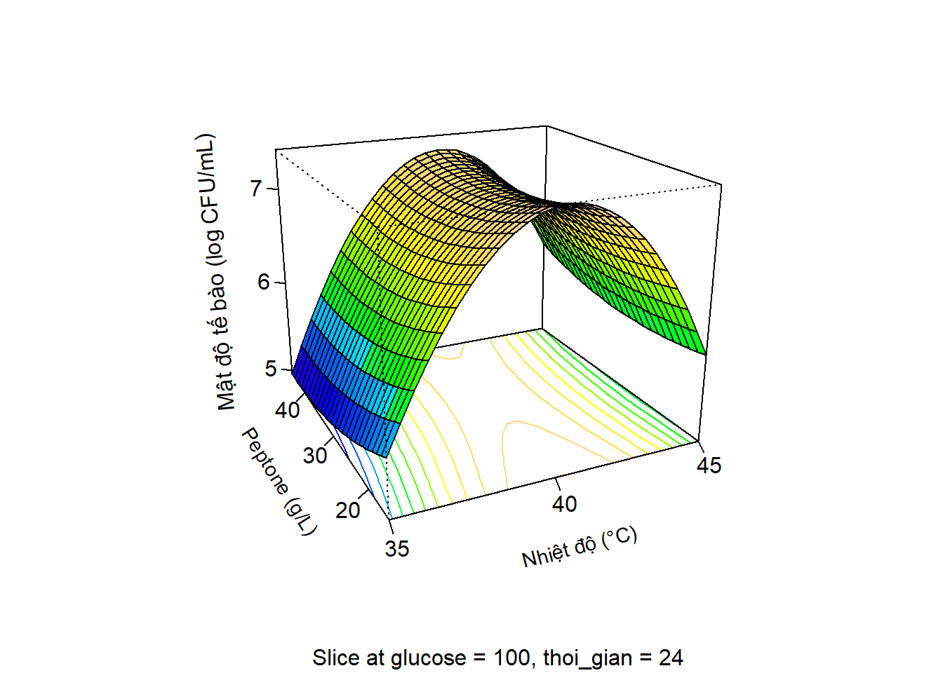
Đồ thị tương quan giữa peptone và nhiệt độ

ok <- persp(
    ket_qua_model,            # Our model
    ~ x1 + x3,    # A formula to obtain the 6 possible graphs
    col = topo.colors(100), # Color palette
    contours = "colors",     # Include contours with the same color palette
    xlabs = c("\n\nNhiệt độ (°C)", 
              "\n\nPeptone (g/L)"), 
    # zlab = "\n\nMật độ tế bào (log CFU/mL)", # Dùng \n để cách hàng
    cex.lab = 0.9,
    expand = 0.8,
    # theta = 30, phi = 30 # Xoay đồ thị,
    ticktype = "detailed",
    nticks = 4
)
par(xpd = NA, srt  = 95)  ## disable clipping and set string rotation
text(-0.28, 0.02,"Mật độ tế bào (log CFU/mL)")

## trích xuất tọa độ x, y, z
ok$`x1 ~ x3`$x -> x
ok$`x1 ~ x3`$y -> y
ok$`x1 ~ x3`$z -> z

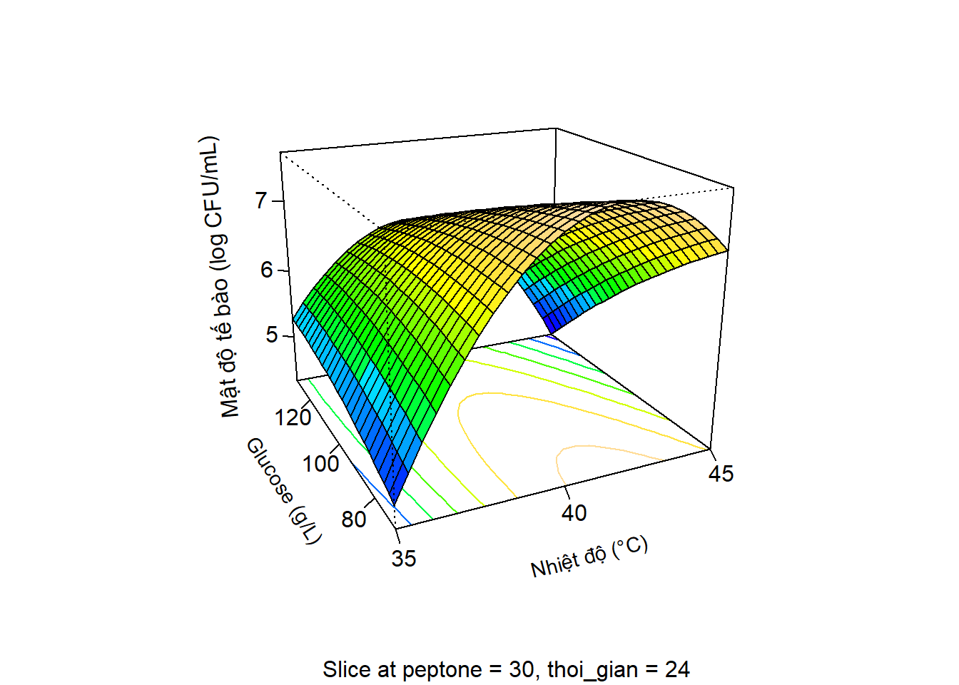
Đồ thị tương quan giữa glucose và nhiệt độ

persp(
    ket_qua_model,            # Our model
    ~ x1 + x2,    # A formula to obtain the 6 possible graphs
    col = topo.colors(100), # Color palette
    contours = "colors",     # Include contours with the same color palette
    xlabs = c("\n\nNhiệt độ (°C)", 
              "\n\nGlucose (g/L)"), 
    # zlab = "\n\nMật độ tế bào (log CFU/mL)", # Dùng \n để cách hàng
    cex.lab = 0.9,
    expand = 0.8,
    # theta = 30, phi = 30 # Xoay đồ thị,
    ticktype = "detailed",
    nticks = 4
)
par(xpd = NA, srt  = 95)  ## disable clipping and set string rotation
text(-0.28, 0.02,"Mật độ tế bào (log CFU/mL)")

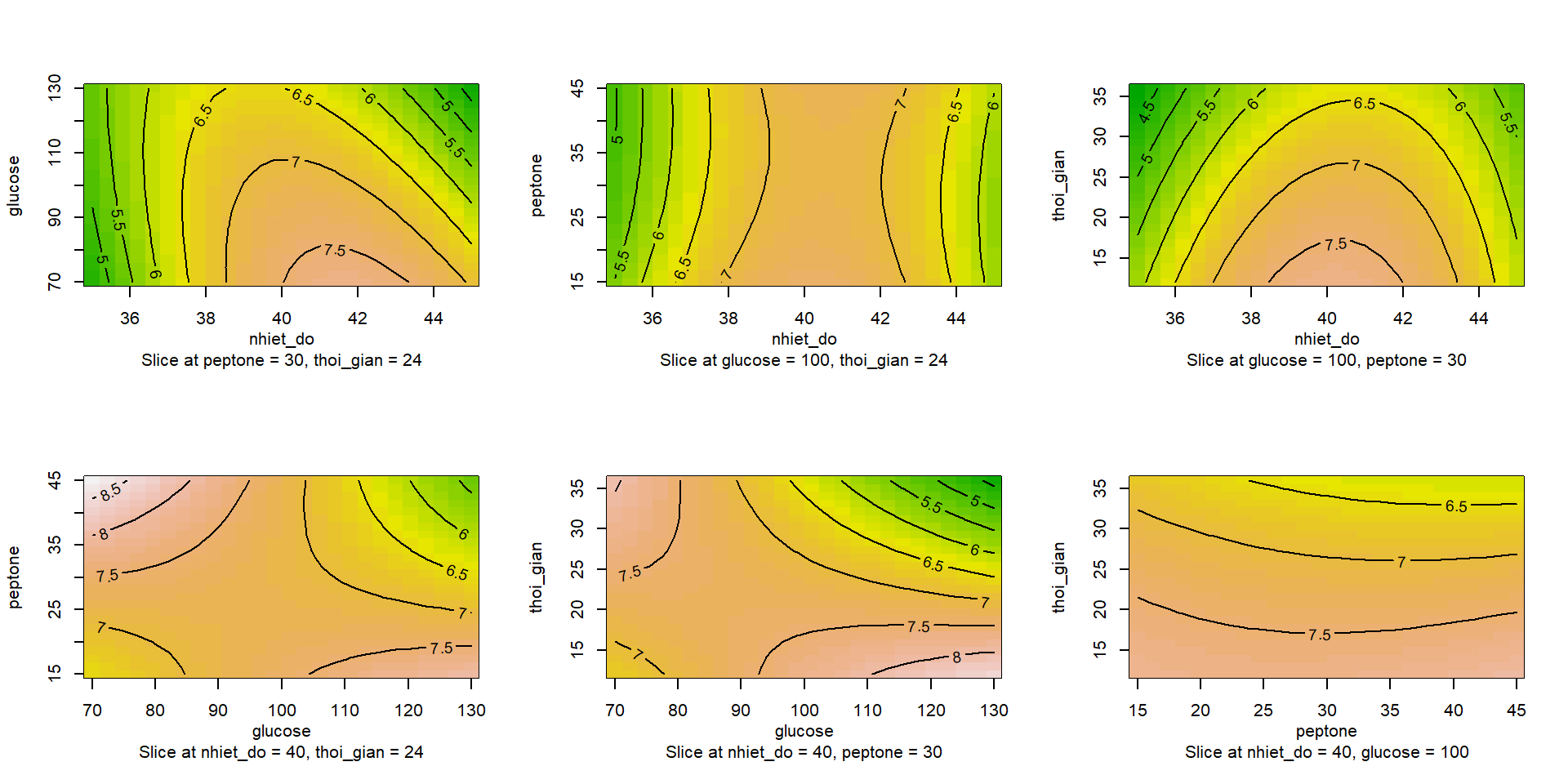
Đồ thị đường đồng mức

par(mfrow = c(2,3))       # 2 x 3 pictures on one plot
contour(
  ket_qua_model,            # Our model
  ~ x1 + x2 + x3 + x4,    # A formula to obtain the 6 possible graphs 
  image = TRUE,           # If image = TRUE, apply color to each contour
  )

Tìm điểm tối ưu

opt_point <- summary(ket_qua_model)$canonical$xs
# opt_point
 
op_point_ru <- code2val(
    opt_point,                     # Optimal point in coded units
    codings = codings(bo_tri_thi_nghiem)  # Formulas to convert to factor units
)
op_point_ru
 nhiet_do   glucose   peptone thoi_gian 
 40.88760  87.06514  13.50203  31.25474 

Dự đoán kết quả đầu ra từ điểm tối ưu

opt_point_df <- data.frame(  # predict() needs a data frame with the points 
    x1 = opt_point[1],         # to be predicted 
    x2 = opt_point[2],
    x3 = opt_point[3],
    x4 = opt_point[4]
)

best_response <- predict(
    ket_qua_model,           # Our model
    opt_point_df             # Data frame with points to be predicted 
)

names(best_response) <- "log_te_bao"
best_response
log_te_bao 
  7.131852 

Kết quả trên có nghĩa là với điều kiện nuôi cấy ở nhiệt độ 40.1 (°C), thời gian 31.3 giờ, sử dụng môi trường nuôi cấy có glucose 87.1 g/L và peptone 13.5 g/L thì sẽ thu được kết quả tối ưu là 7.13 log CFU/mL hay là 1.3 × 10⁷ CFU/mL.

16.0.3.1 Tài liệu tham khảo

  1. https://cran.r-project.org/web/packages/plot3D/

  2. http://www.sthda.com/english/wiki/impressive-package-for-3d-and-4d-graph-r-software-and-data-visualization

  3. https://plotly.com/r/3d-surface-plots/