Example dataset
Sử dụng ví dụ ở chapter 10 trong cuốn sách này.
https://studyr.netlify.app/ref/introductory_biostatistics_2016.pdf
cancer <- read.csv("prostatecancer.dat", sep = "&")
cancer
   Xray Grade Stage Age Acid Nodes
1     0     1     1  64   40     0
2     0     0     1  63   40     0
3     1     0     0  65   46     0
4     0     1     0  67   47     0
5     0     0     0  66   48     0
6     0     1     1  65   48     0
7     0     0     0  60   49     0
8     0     0     0  51   49     0
9     0     0     0  66   50     0
10    0     0     0  58   50     0
11    0     1     0  56   50     0
12    0     0     1  61   50     0
13    0     1     1  64   50     0
14    0     0     0  56   52     0
15    0     0     0  67   52     0
16    1     0     0  49   55     0
17    0     1     1  52   55     0
18    0     0     0  68   56     0
19    0     1     1  66   59     0
20    1     0     0  60   62     0
21    0     0     0  61   62     0
22    1     1     1  59   63     0
23    0     0     0  51   65     0
24    0     1     1  53   66     0
25    0     0     0  58   71     0
26    0     0     0  63   75     0
27    0     0     1  53   76     0
28    0     0     0  60   78     0
29    0     0     0  52   83     0
30    0     0     1  67   95     0
31    0     0     0  56   98     0
32    0     0     1  61  102     0
33    0     0     0  64  187     0
34    1     0     1  58   48     1
35    0     0     1  65   49     1
36    1     1     1  57   51     1
37    0     1     0  50   56     1
38    1     1     0  67   67     1
39    0     0     1  67   67     1
40    0     1     1  57   67     1
41    0     1     1  45   70     1
42    0     0     1  46   70     1
43    1     0     1  51   72     1
44    1     1     1  60   76     1
45    1     1     1  56   78     1
46    1     1     1  50   81     1
47    0     0     0  56   82     1
48    0     0     1  63   82     1
49    1     1     1  65   84     1
50    1     0     1  64   89     1
51    0     1     0  59   99     1
52    1     1     1  68  126     1
53    1     0     0  61  136     1
Logistic Regression Model
Effect of Measurement Scale
acid.glm <- glm(Nodes ~ Acid,
                data = cancer,
                family = binomial(link = "logit"))
# acid.glm

summary(acid.glm)
Call:
glm(formula = Nodes ~ Acid, family = binomial(link = "logit"),
    data = cancer)

Coefficients:
            Estimate Std. Error z value Pr(>|z|)
(Intercept) -1.92703    0.92104  -2.092   0.0364 *
Acid         0.02040    0.01257   1.624   0.1045
---
Signif. codes:  0 '***' 0.001 '**' 0.01 '*' 0.05 '.' 0.1 ' ' 1

(Dispersion parameter for binomial family taken to be 1)

    Null deviance: 70.252  on 52  degrees of freedom
Residual deviance: 67.116  on 51  degrees of freedom
AIC: 71.116

Number of Fisher Scoring iterations: 4
or.50acid <- exp((100-50)*acid.glm$coefficients[2])

or.50acid
Testing Hypotheses in Multiple Logistic Regression
all.glm <- glm(Nodes ~ Xray + Grade + Stage + Age + Acid,
              data = cancer,
              family = binomial(link = "logit"))

summary(all.glm)
Call:
glm(formula = Nodes ~ Xray + Grade + Stage + Age + Acid, family = binomial(link = "logit"),
    data = cancer)

Coefficients:
            Estimate Std. Error z value Pr(>|z|)
(Intercept)  0.06180    3.45992   0.018   0.9857
Xray         2.04534    0.80718   2.534   0.0113 *
Grade        0.76142    0.77077   0.988   0.3232
Stage        1.56410    0.77401   2.021   0.0433 *
Age         -0.06926    0.05788  -1.197   0.2314
Acid         0.02434    0.01316   1.850   0.0643 .
---
Signif. codes:  0 '***' 0.001 '**' 0.01 '*' 0.05 '.' 0.1 ' ' 1

(Dispersion parameter for binomial family taken to be 1)

    Null deviance: 70.252  on 52  degrees of freedom
Residual deviance: 48.126  on 47  degrees of freedom
AIC: 60.126

Number of Fisher Scoring iterations: 5
chisq.LR <- all.glm$null.deviance - all.glm$deviance

chisq.LR
df.LR <- all.glm$df.null - all.glm$df.residual

df.LR
Stepwise
library(MASS)
MASS::stepAIC(all.glm)
Start:  AIC=60.13
Nodes ~ Xray + Grade + Stage + Age + Acid

        Df Deviance    AIC
- Grade  1   49.097 59.097
- Age    1   49.615 59.615
<none>       48.126 60.126
- Acid   1   51.572 61.572
- Stage  1   52.558 62.558
- Xray   1   55.350 65.350

Step:  AIC=59.1
Nodes ~ Xray + Stage + Age + Acid

        Df Deviance    AIC
- Age    1   50.660 58.660
<none>       49.097 59.097
- Acid   1   52.085 60.085
- Stage  1   55.381 63.381
- Xray   1   57.016 65.016

Step:  AIC=58.66
Nodes ~ Xray + Stage + Acid

        Df Deviance    AIC
<none>       50.660 58.660
- Acid   1   53.353 59.353
- Stage  1   57.059 63.059
- Xray   1   58.613 64.613
Call:  glm(formula = Nodes ~ Xray + Stage + Acid, family = binomial(link = "logit"),
    data = cancer)

Coefficients:
(Intercept)         Xray        Stage         Acid
   -3.57565      2.06179      1.75556      0.02063

Degrees of Freedom: 52 Total (i.e. Null);  49 Residual
Null Deviance:      70.25
Residual Deviance: 50.66    AIC: 58.66
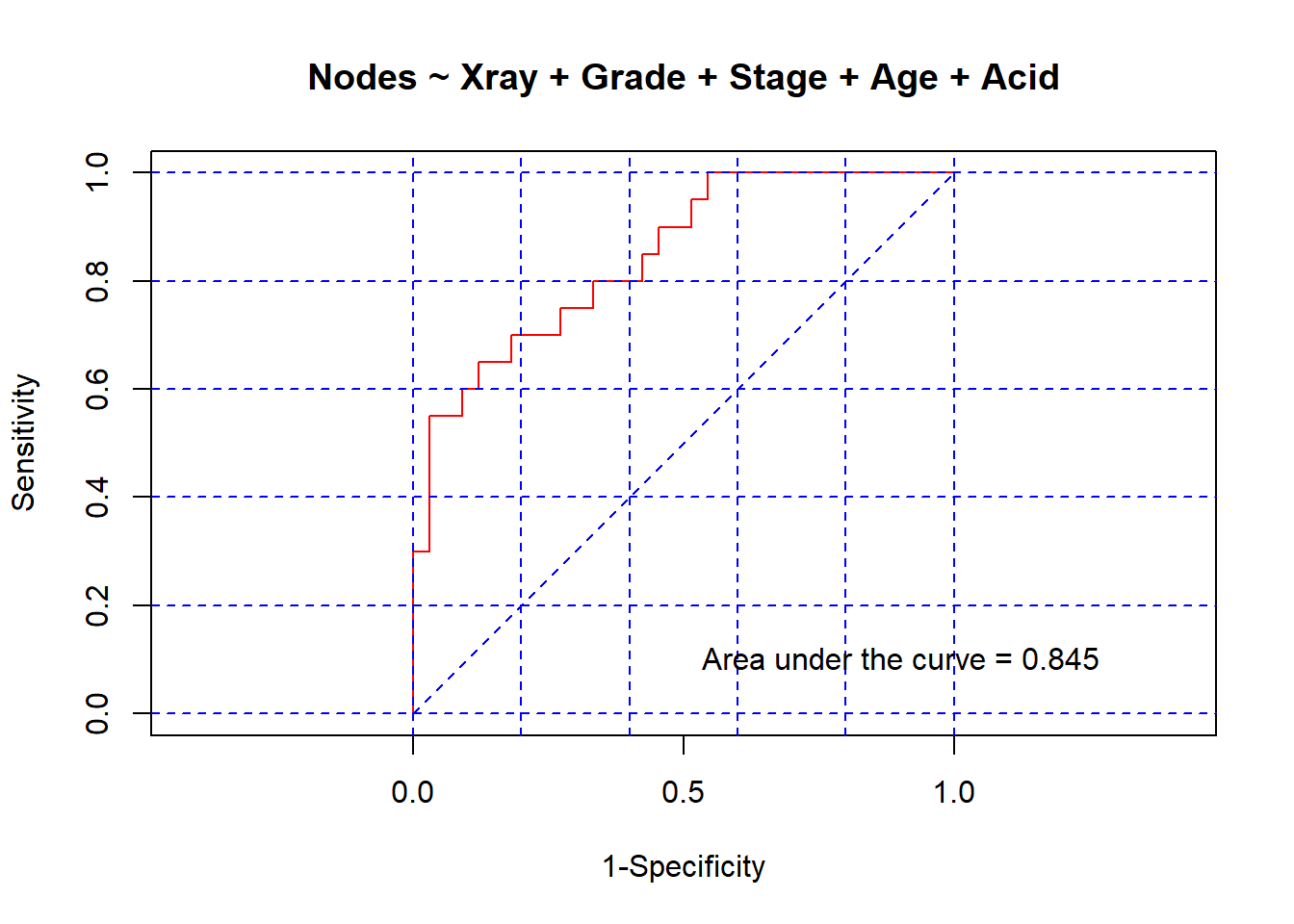
ROC curve
Loading required package: foreign
Loading required package: survival
Attaching package: 'survival'
The following object is masked _by_ '.GlobalEnv':

    cancer
Loading required package: nnet
all.glm.roc <- lroc(all.glm, title = TRUE, auc.coords = c(0.5, 0.1))
$model.description
[1] "Nodes ~ Xray + Grade + Stage + Age + Acid"

$auc
[1] 0.8454545

$predicted.table
 predicted.prob Non-diseased Diseased
         0.0341            1        0
         0.0351            1        0
         0.0358            1        0
         0.0361            1        0
         0.0521            1        0
         0.0607            1        0
         0.0645            1        0
         0.0657            1        0
         0.0723            1        0
         0.0775            1        0
         0.0929            1        0
         0.0973            1        0
         0.1002            1        0
         0.1314            1        0
         0.1372            1        0
         0.1393            0        1
         0.1463            1        0
         0.1566            0        1
         0.1795            1        0
         0.1929            1        0
         0.2004            0        1
         0.2007            1        0
         0.2181            0        1
         0.2184            1        0
         0.2551            1        0
         0.2796            1        0
         0.2988            0        1
         0.3040            1        0
         0.3213            1        0
         0.3227            0        1
         0.3314            1        0
         0.3684            1        0
         0.4514            1        0
         0.4648            0        1
         0.4710            1        0
         0.5130            1        0
         0.5176            0        1
         0.5311            1        0
         0.5359            0        1
         0.5452            1        0
         0.5801            1        0
         0.6948            0        1
         0.7260            0        1
         0.7673            0        1
         0.8030            0        1
         0.8489            0        1
         0.8676            1        0
         0.8689            0        1
         0.8782            0        1
         0.8935            0        1
         0.9207            0        1
         0.9421            0        1
         0.9498            0        1

$diagnostic.table
   1-Specificity Sensitivity
      1.00000000        1.00
>     0.96969697        1.00
>     0.93939394        1.00
>     0.90909091        1.00
>     0.87878788        1.00
>     0.84848485        1.00
>     0.81818182        1.00
>     0.78787879        1.00
>     0.75757576        1.00
>     0.72727273        1.00
>     0.69696970        1.00
>     0.66666667        1.00
>     0.63636364        1.00
>     0.60606061        1.00
>     0.57575758        1.00
>     0.54545455        1.00
>     0.54545455        0.95
>     0.51515152        0.95
>     0.51515152        0.90
>     0.48484848        0.90
>     0.45454545        0.90
>     0.45454545        0.85
>     0.42424242        0.85
>     0.42424242        0.80
>     0.39393939        0.80
>     0.36363636        0.80
>     0.33333333        0.80
>     0.33333333        0.75
>     0.30303030        0.75
>     0.27272727        0.75
>     0.27272727        0.70
>     0.24242424        0.70
>     0.21212121        0.70
>     0.18181818        0.70
>     0.18181818        0.65
>     0.15151515        0.65
>     0.12121212        0.65
>     0.12121212        0.60
>     0.09090909        0.60
>     0.09090909        0.55
>     0.06060606        0.55
>     0.03030303        0.55
>     0.03030303        0.50
>     0.03030303        0.45
>     0.03030303        0.40
>     0.03030303        0.35
>     0.03030303        0.30
>     0.00000000        0.30
>     0.00000000        0.25
>     0.00000000        0.20
>     0.00000000        0.15
>     0.00000000        0.10
>     0.00000000        0.05
>     0.00000000        0.00