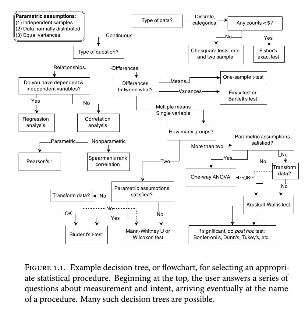
Để làm rõ về quy trình phân tích theo hai hướng parametric (có các tham số như trung bình và phương sai của phân bố chuẩn) và non-parametric (không có các tham số cho phân bố chuẩn) ta sẽ xét cách làm trên cùng 1 bộ dataset.
Dataset minh họa: Dữ liệu đo khối lượng cây ở các nghiệm thức khác nhau.
Giả thuyết:
\({H_0}\) : Giữa các nghiệm thức không khác nhau về khối lượng cây
\({H_\alpha }\) : Giữa các nghiệm thức khác nhau về khối lượng cây
library(tidyverse)library(ggpubr)library(rstatix)### sửa lại dữ liệu từ dataset PlantGrowth để trở thành dữ liệu không có phân bố chuẩn.PlantGrowth -> dfdf[1, 1] <-6.39df[2, 1] <-6.14df[3, 1] <-7.39df[4, 1] <-7.55df[5, 1] <-9.32df[6, 1] <-8.39df[21, 1] <-1.39df[22, 1] <-1.14df[23, 1] <-1.39df[24, 1] <-0.55df[25, 1] <-1.32df[12, 1] <-2.39df[13, 1] <-1.14df[14, 1] <-1.39df[15, 1] <-0.55df[16, 1] <-1.32df
# A tibble: 3 × 6
  group count  mean    sd median   IQR
  <fct> <int> <dbl> <dbl>  <dbl> <dbl>
1 ctrl     10  6.54  1.58   6.26  2.3
2 trt1     10  3.15  1.99   3.36  3.44
3 trt2     10  3.32  2.32   3.16  3.95
df %>%group_by(group) %>% ggpubr::get_summary_stats(weight, type ="common")
# A tibble: 3 × 11
  group variable     n   min   max median   iqr  mean    sd    se    ci
  <fct> <fct>    <dbl> <dbl> <dbl>  <dbl> <dbl> <dbl> <dbl> <dbl> <dbl>
1 ctrl  weight      10  4.53  9.32   6.26  2.3   6.54  1.58 0.499  1.13
2 trt1  weight      10  0.55  6.03   3.36  3.44  3.15  1.99 0.629  1.42
3 trt2  weight      10  0.55  6.15   3.16  3.94  3.32  2.32 0.732  1.66
11.0.2Bước 2: Phân tích ANOVA 1 yếu tố cho trường hợp parametric
Tham khảo: https://www.statsmadeasy.com/tutorial-4-inferential-stats-test-of-difference/one-way-anova-parametric-non-parametric
Bước 2.1: Parametric One-Way ANOVA Assumptions
Independence: Your observations in each sample should be independent. \(\Rightarrow\) OK
Independent Variable: This variable must have 3 or more outcomes. (mỗi chỉ tiêu cần đo lặp lại ít nhất 3 lần) \(\Rightarrow\) OK
Random Sampling: Your data should be a random sample of the target population. \(\Rightarrow\) OK
Equal Variance (Homogeneity): Both groups should have approximately the same variance.
Normality: Your Dependent variable should be approximately normally distributed.
Bước 2.2: Kiểm tra giả thuyết
# Kiểm tra giả thuyết Normalityres.aov <-aov(weight ~ group, data = df)aov_residuals <-residuals(object = res.aov)shapiro.test(x = aov_residuals)
    Shapiro-Wilk normality test

data:  aov_residuals
W = 0.88797, p-value = 0.00432
Kết quả Shapiro-Wilk normality test cho thấy p-value là 0.00432 nhỏ hơn 0.05. Do đó bộ dataset này KHÔNG phân bố chuẩn. \(\Rightarrow\) VIOLATE
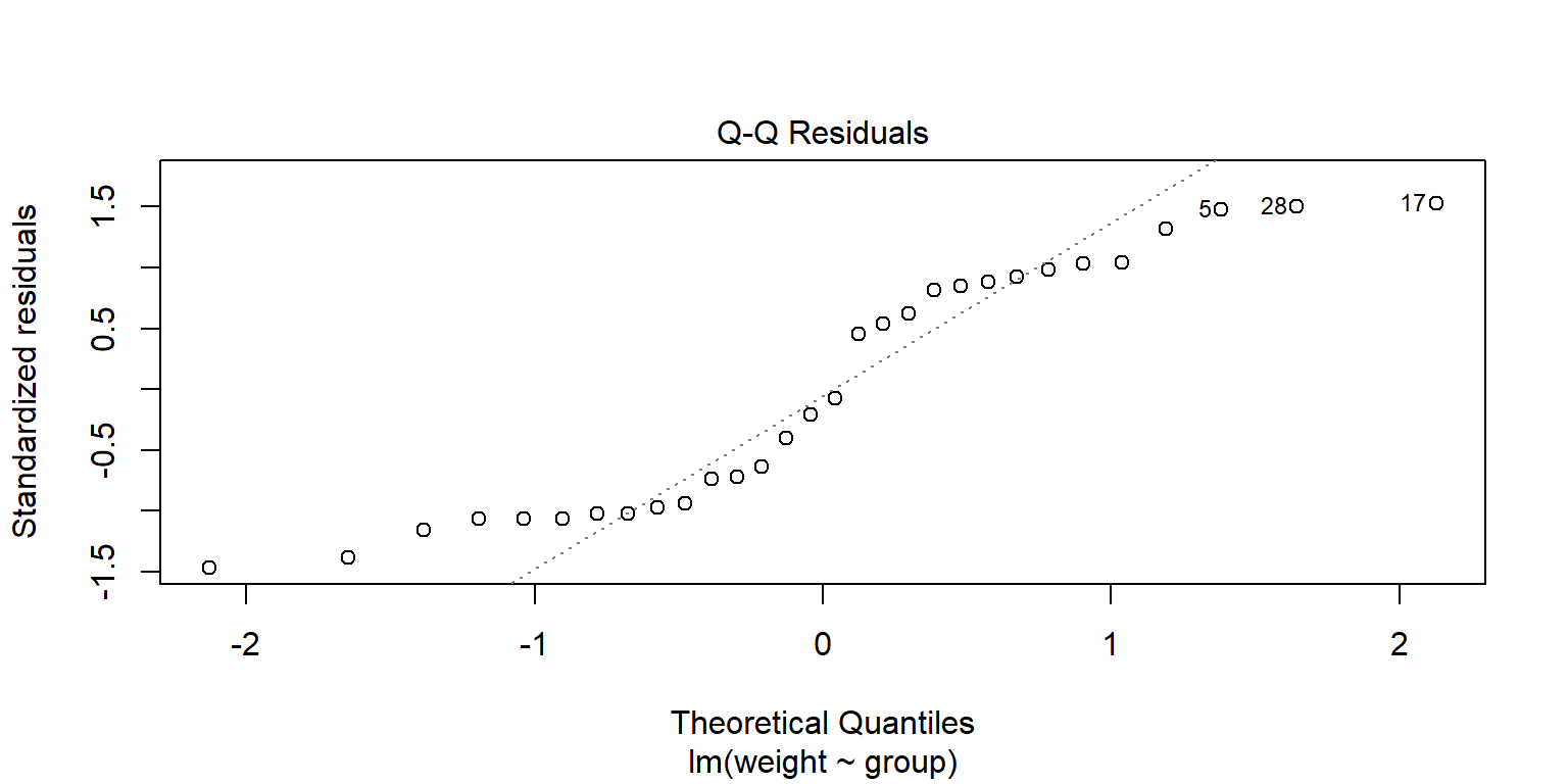
# Kiểm tra giả thuyết Normality qua Q-Q plotmod <-lm(weight ~ group, data = df)plot(mod, 2)
Nhìn đồ thị Q-Q lot ta thấy các giá trị không có phân bố chuẩn.
# Kiểm tra giả thuyết Equal Variance (Homogeneity)library(car)leveneTest(weight ~ group, data = df)
Levene's Test for Homogeneity of Variance (center = median)
      Df F value  Pr(>F)
group  2  4.3203 0.02356 *
      27
---
Signif. codes:  0 '***' 0.001 '**' 0.01 '*' 0.05 '.' 0.1 ' ' 1
Kết quả Levene’s test cho thấy p-value là 0.02356 nhỏ hơn 0.05. Do đó bộ dataset này có sự khác biệt về phương sai giữa các tổ hợp các mức khác nhau của 2 biến \(\Rightarrow\) VIOLATE
It’s also possible to use Bartlett’s test or Levene’s test to check the homogeneity of variances.
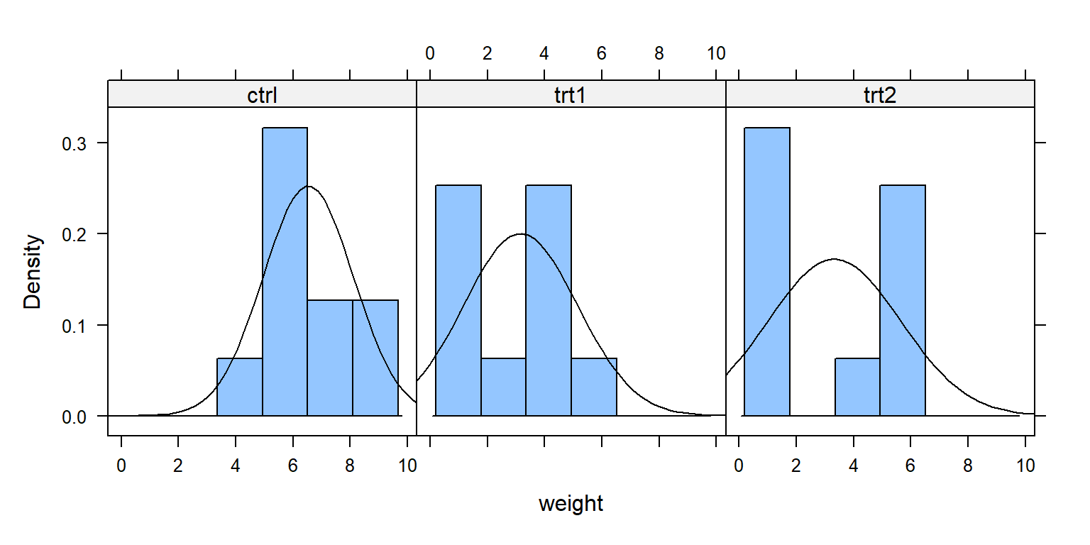
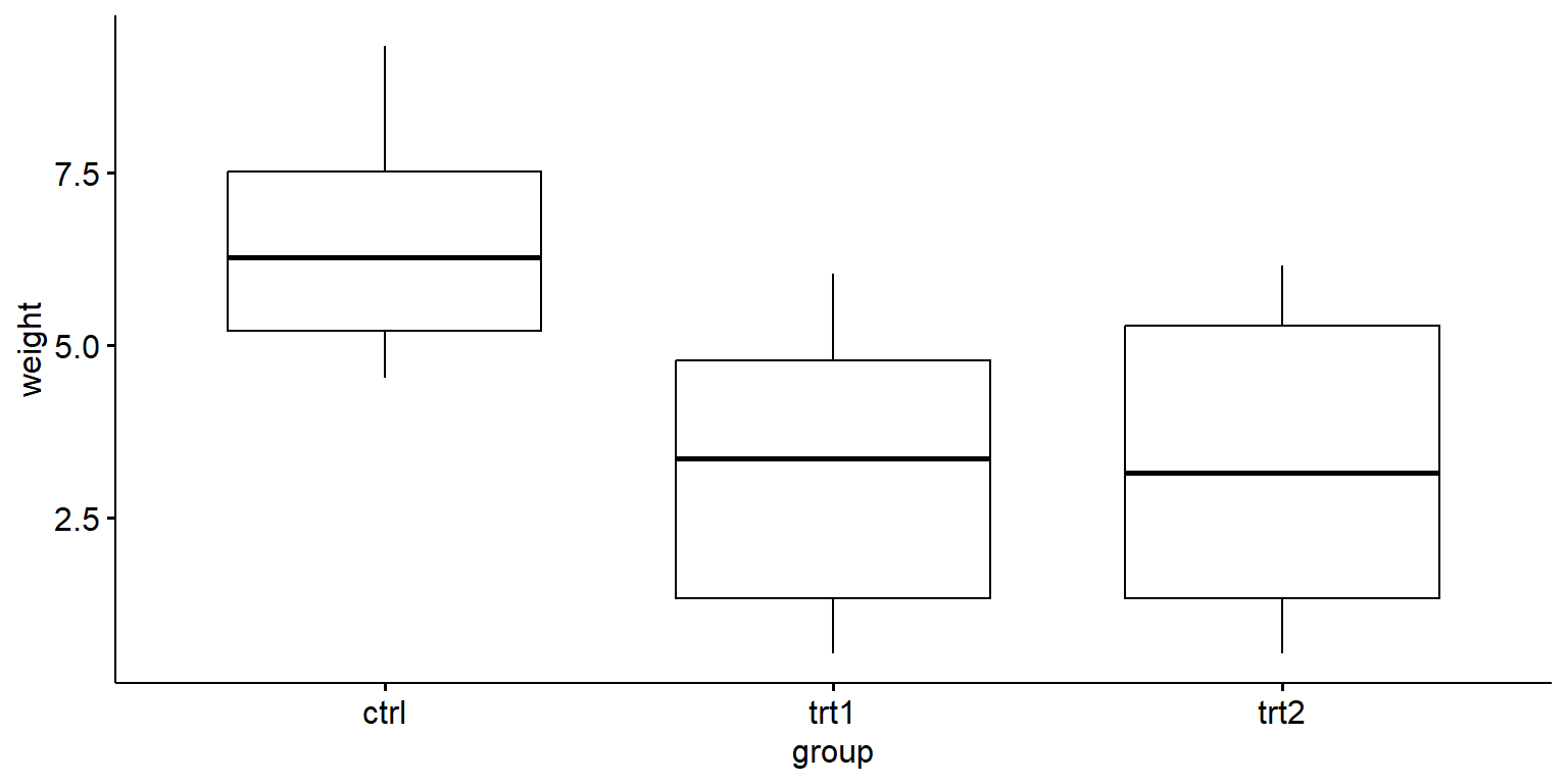
Bước 2.3: Mô tả đặc điểm dữ liệu qua đồ thị
library(lattice)histogram( ~ weight | group, data =df,type ="density",panel =function(x, ...) {panel.histogram(x, ...)panel.mathdensity(dmath = dnorm, col ="black",args =list(mean=mean(x),sd=sd(x))) } )
###ggpubr::ggboxplot(df, x ="group", y ="weight")
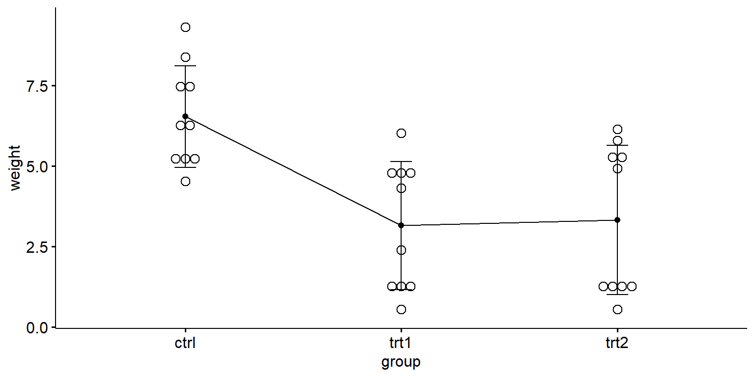
ggpubr::ggline(df, x ="group", y ="weight", order =c("ctrl", "trt1", "trt2"), add =c("mean_sd", "dotplot"))
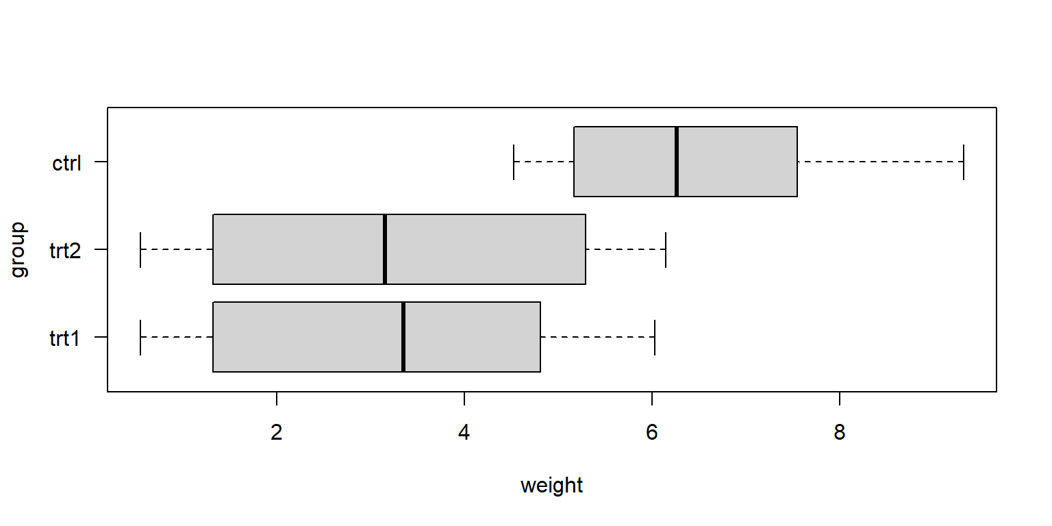
###df$group <-reorder(df$group, df$weight, decreasing =FALSE) boxplot(weight ~ group, data = df, frame =TRUE,horizontal =TRUE, las =1,axisnames =TRUE)
Bước 2.4: Thực hiện ANOVA 1 yếu tố
Cho dù đã vi phạm giả thuyết, nếu ta vẫn tiếp tục thực hiện ANOVA 1 yếu tố như bình thường thì kết quả sẽ như sau.
res.aov <-aov(weight ~ group, data = df)anova(res.aov)
Analysis of Variance Table

Response: weight
          Df  Sum Sq Mean Sq F value    Pr(>F)
group      2  72.653  36.327  9.2271 0.0008834 ***
Residuals 27 106.298   3.937
---
Signif. codes:  0 '***' 0.001 '**' 0.01 '*' 0.05 '.' 0.1 ' ' 1
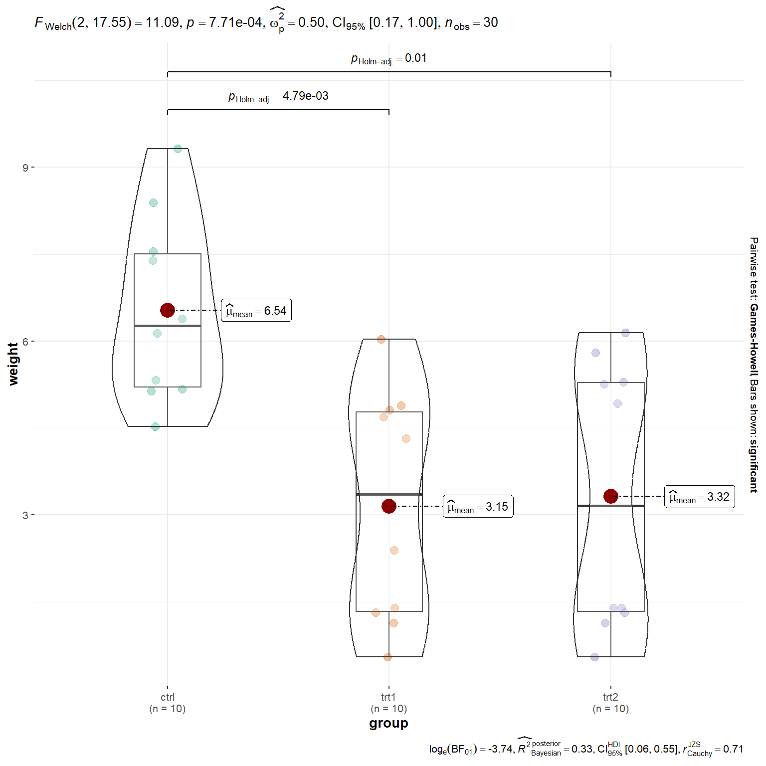
Kết quả cho thấy p-value = 0.0008834 nhỏ hơn 0.05 nên có ý nghĩa thống kê, dù rằng dataset này đã vi phạm giả thuyết về phân bố chuẩn!
Tham khảo thêm:
ANOVA test with no assumption of equal variances
oneway.test(weight ~ group, data = df)
    One-way analysis of means (not assuming equal variances)

data:  weight and group
F = 11.087, num df = 2.000, denom df = 17.548, p-value = 0.0007708
Pairwise t-tests with no assumption of equal variances
    Pairwise comparisons using t tests with non-pooled SD

data:  df$weight and df$group

     trt1   trt2
trt2 0.8638 -
ctrl 0.0017 0.0034

P value adjustment method: BH
Study: res.aov ~ "group"
HSD Test for weight
Mean Square Error: 3.936961
group, means
weight std r se Min Max Q25 Q50 Q75
ctrl 6.535 1.578215 10 0.6274521 4.53 9.32 5.2100 6.265 7.5100
trt1 3.153 1.990037 10 0.6274521 0.55 6.03 1.3375 3.355 4.7800
trt2 3.321 2.315141 10 0.6274521 0.55 6.15 1.3375 3.155 5.2825
Alpha: 0.05 ; DF Error: 27
Critical Value of Studentized Range: 3.506426
Minimun Significant Difference: 2.200114
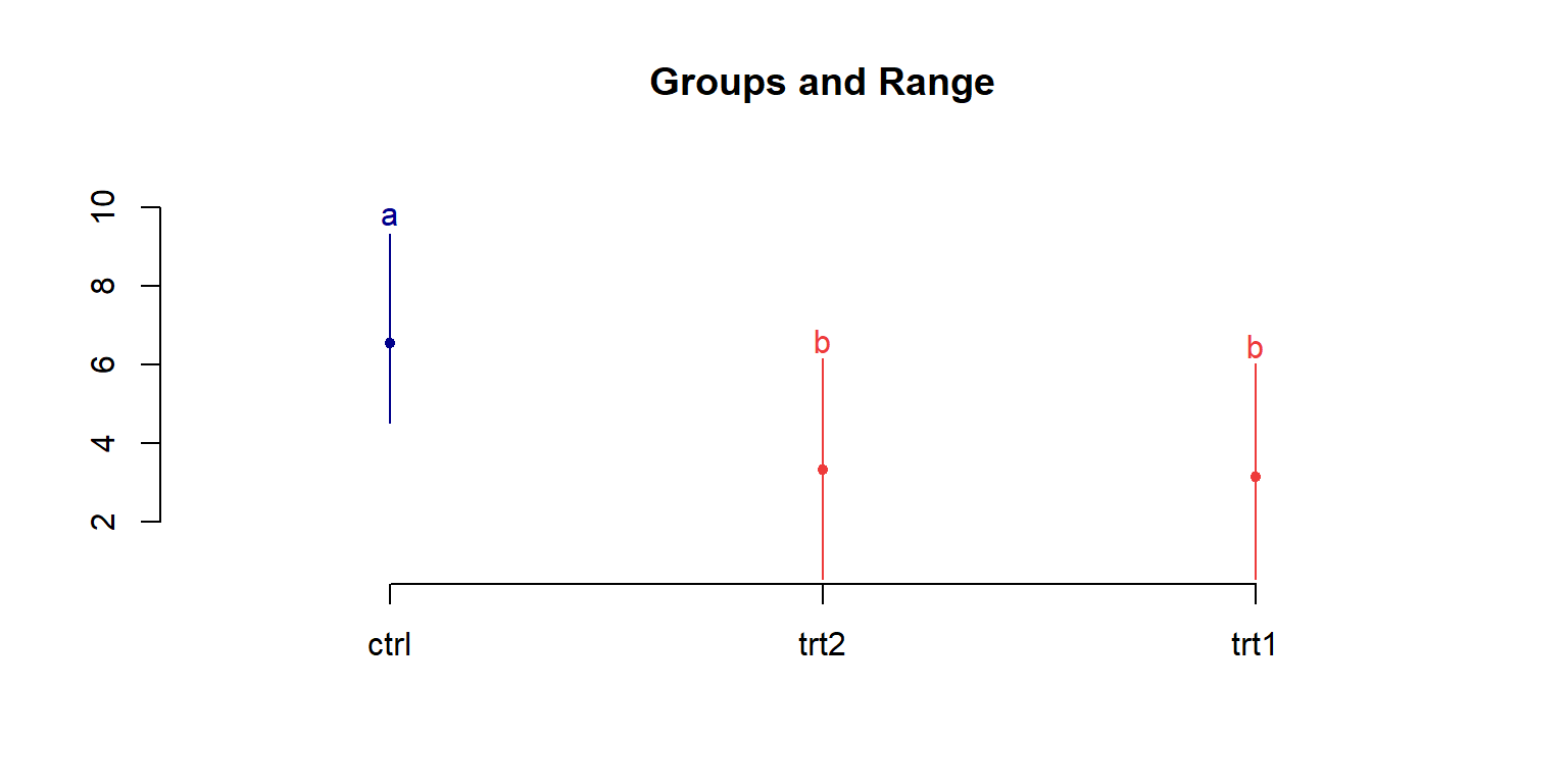
Treatments with the same letter are not significantly different.
weight groups
ctrl 6.535 a
trt2 3.321 b
trt1 3.153 b
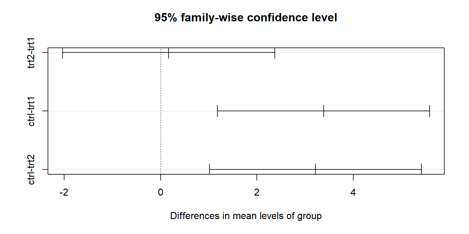
plot(tukey_ok)
Kết quả cho thấy vẫn thực hiện được phân hạng theo Tukey như bình thường, dù rằng dataset này đã vi phạm giả thuyết về phân bố chuẩn!
# A tibble: 1 × 6
.y. n statistic df p method
* <chr> <int> <dbl> <int> <dbl> <chr>
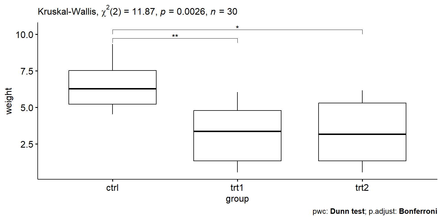
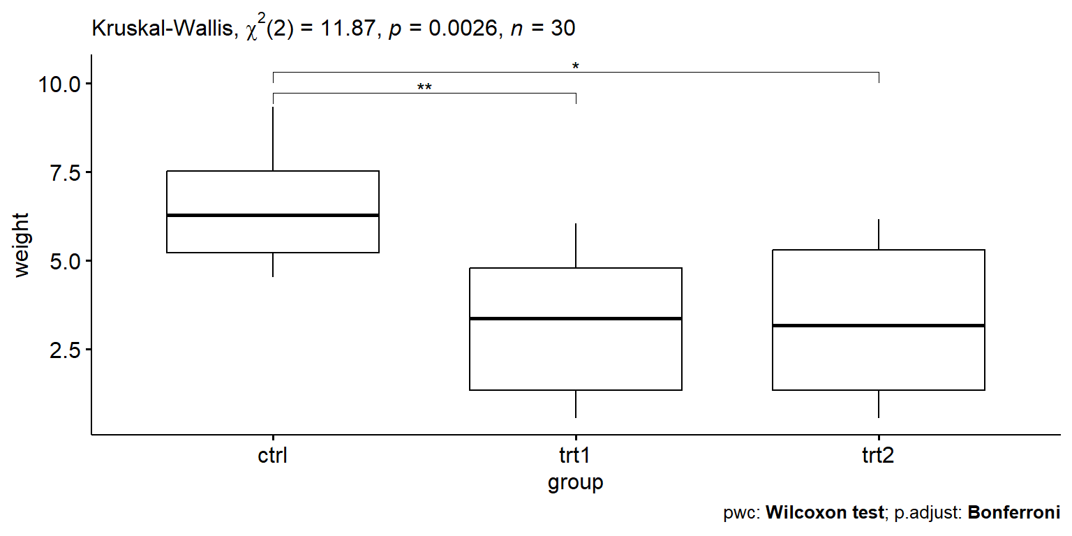
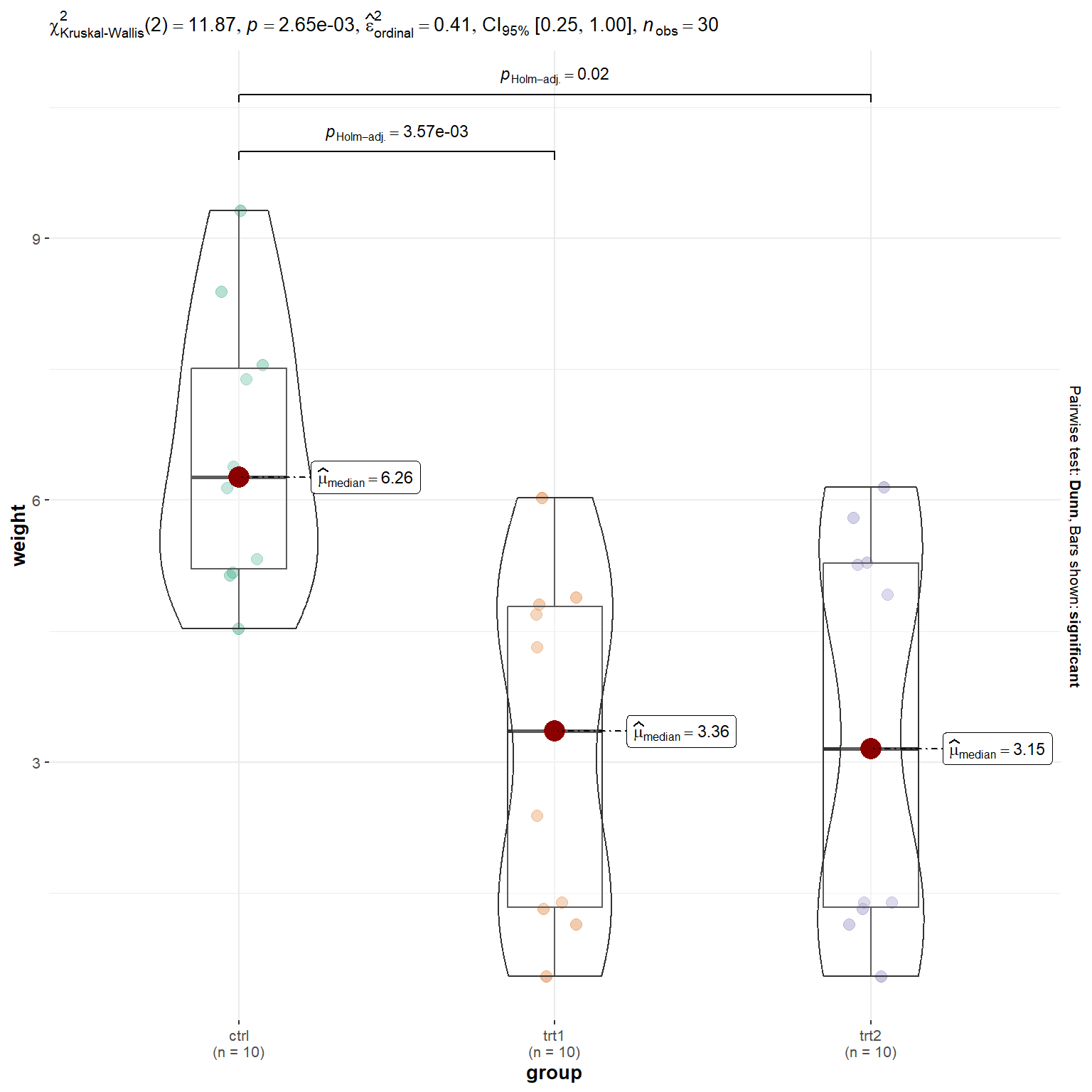
1 weight 30 11.9 2 0.00265 Kruskal-Wallis
Kết quả cho thấy p-value = 0.00265 nhỏ hơn 0.05 nên có ý nghĩa thống kê. Đây cũng trùng hợp với kết quả từ ANOVA parametric ở trên!
Về lý thuyết, Kruskal-Wallis test có thể áp dụng cho two groups. Nhưng trong thực tế ta sẽ dùng the Mann-Whitney test for two groups and Kruskal-Wallis for three or more groups.
The eta squared, based on the H-statistic, can be used as the measure of the Kruskal-Wallis test effect size. It is calculated as follow : eta2[H] = (H - k + 1)/(n - k); where H is the value obtained in the Kruskal-Wallis test; k is the number of groups; n is the total number of observations (M. T. Tomczak and Tomczak 2014).
The eta-squared estimate assumes values from 0 to 1 and multiplied by 100 indicates the percentage of variance in the dependent variable explained by the independent variable.
The interpretation values commonly in published literature are: 0.01- < 0.06 (small effect), 0.06 - < 0.14 (moderate effect) and >= 0.14 (large effect).
df |> rstatix::kruskal_effsize(weight ~ group)
# A tibble: 1 × 5
  .y.        n effsize method  magnitude
* <chr>  <int>   <dbl> <chr>   <ord>
1 weight    30   0.365 eta2[H] large
Ý nghĩa của effect size
https://lbecker.uccs.edu/glm_effectsize
Bước 3.5: Phân hạng trong trường hợp non-parametric
Lưu ý: Phân hạng theo parametric (Tukey’s test) thì ta căn cứ vào mean nên tính được diff mean (sự khác biệt giữa các trung bình) nên có thể phân ra theo từng hạng a, b, c, … còn phân hạng theo non-parametric ta căn cứ vào median nên chỉ phân hạng theo từng cặp, theo sign test +/- cho thấy sự khác biệt giữa các cặp nghiệm thức với nhau.
Cách 1: Pairwise comparisons using Dunn’s test (most common post-hoc test)
Kết quả so sánh theo cặp theo Dunn’s test cho thấy cặp nghiệm thức trt1-trt2 không khác nhau về mặt ý nghĩa thống kê p-value là ns. Còn lại giữa 2 cặp nghiệm thức ctrl-trt1 và ctrl-trt2 khác biệt có ý nghĩa thống kê vì p-value nhỏ hơn 0.05.
Cách 2: Pairwise comparisons using Dunn’s test trong package FSA
# Note that there are other p-value adjustment methods. See ?dunnTest for more options
It is the last column (the adjusted p-values, adjusted for multiple comparisons) that is of interest. These p-values should be compared to your desired significance level (usually 5%).
Based on the output, we conclude that:
ctrl and trt1 differ significantly (p < 0.05)
ctrl and trt2 differ significantly (p < 0.05)
trt1 and trt2 NOT differ significantly (p > 0.05)
Therefore, based on the Dunn’s test, we can now conclude that only ctrl-trt1 and ctrl-trt2 differ in terms of weight.
Cách 3: Pairwise comparisons using Wilcoxon’s test
Kết quả so sánh theo cặp theo Wilcoxon’s test cho thấy cặp nghiệm thức trt1-trt2 không khác nhau về mặt ý nghĩa thống kê p-value là ns. Còn lại giữa 2 cặp nghiệm thức ctrl-trt1 và ctrl-trt2 khác biệt có ý nghĩa thống kê vì p-value nhỏ hơn 0.05.
Cách 3: Thể hiện phân hạng qua đồ thị boxplot
## Dunn's testpwc <- pwc %>%add_xy_position(x ="group")ggboxplot(df, x ="group", y ="weight") +stat_pvalue_manual(pwc, hide.ns =TRUE) +labs(subtitle =get_test_label(res.kruskal, detailed =TRUE),caption =get_pwc_label(pwc) )
# Wilcoxon's testpwc2 <- pwc2 %>%add_xy_position(x ="group")ggboxplot(df, x ="group", y ="weight") +stat_pvalue_manual(pwc2, hide.ns =TRUE) +labs(subtitle =get_test_label(res.kruskal, detailed =TRUE),caption =get_pwc_label(pwc2) )